Deep Learning

18 Jun 2019

This series of posts on Deep learning is my notes on Deep learning from the course 6.S191 Introduction to Deep Learning. It is meant to be more of a personal notes so if you find something less descriptive please follow this link.

The Perceptron

Structural building blocks

A Perceptron is the fundamental building block of neural networks. The idea of Perceptron’s can be traced back to the functioning of a Neuron in animals, i.e. when activated it fires a pulse of current. Similarly, a Perceptron usually takes input, multiplies it with a weight and squashes it with a activation function, which can be represented via the following equation.

\[\begin{align*} \hat{y} = g \left(w_0 + \sum_{i=1}^n w_ix_i \right) \end{align*}\]

Where \(\hat{y}\) is the output, \(g(\cdot)\) is the activation function, \(n\) is the number of inputs, \(w_i\) are the respective weights for the input \(x_i\) and \(w_0\) is the bias.

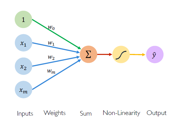fig: A Perceptron

The vectorial representation of the above equation is given by

\[\begin{align*} \hat{y} = g \left(w_0 + \bf{X^TW} \right) \end{align*}\]

The activation function \(g(\cdot)\) used are usually a non-linear activation function. A example of a non-linear activation function is the sigmoid function which is given by.

\[\begin{align*} g(z) = \sigma(z) = \frac{1}{1 + e^{-z}} \end{align*}\]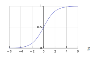

sigmid_function fig: A sigmoid activation function

Nonlinear activation functions

Why a Non-linear activation function? The whole purpose of activation function is tp introduce non-linearities to the network. A linear activation function produces a linear decision boundary. As we know all the real world systems are non-linear it makes much sense to use a non-linear activation function.

Here are some activation functions with their use code in Tensorflow.

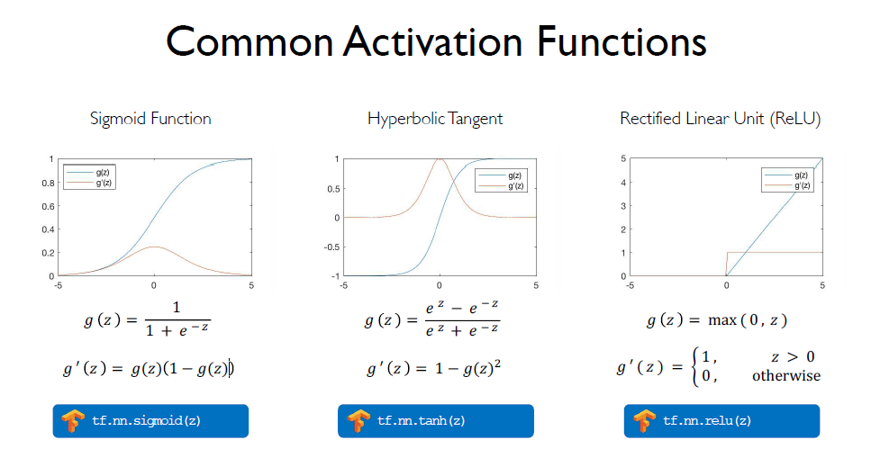activaion_functions fig: Common activation functions

Neural Networks

Although a single perceptron can work as a classifier on its own, it cannot generalise well and leran complex features of problems. Thus the need to have a neural network which is constructed by stacking units of perceptron together.

Stacking Perceptrons to form neural networks

Here is a example of a multi-output Perceptrons.

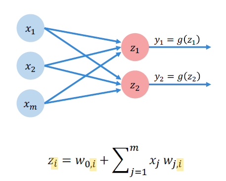multi_output_perceptron fig: A Multi-output Perceptron

A Feed Forward Neural Network is a network with layers of perceptron connected from one layer to another. Here is an example of a Neural Network with a input layer connected to a hidden layer, which is then connected to a output layer which contains multiple output. This is called as a single layer Neural Network.

single_layer_neural_network 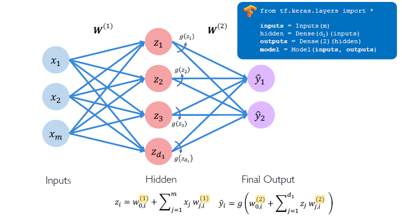fig: A single layer Neural Network

A Deep Neural Network is made up of many hidden layers which picks up a different types of feature in each of its hidden layers.

Optimization through backpropagation

A randomly initialized Neural Network given a task performs poorly. To teach a NN to perform better we have to quantify the error with respect to training data that it is trying to learn the underlying features of. This we can do by constructing a Loss function, with which we can compute a cost function by which we can update the weights that are initialized.

\[\begin{align*} J(W) = \frac{1}{n} \sum_{i=1}^n L \left(f(x^{(i)};W), y^{(i)} \right) \end{align*}\]

Here \(J(W)\) is the cost function, and \(L (f(x^{(i)};W), y^{(i)}\) is the loss function of the \(i^{th}\) input and output.

Here are two Cost functions commonly used in pracice.

Binary Cross Entropy Loss

Cross entropy loss can be used with models that output a probability between 0 and 1.

\[\begin{align*} J(W) = \frac{1}{n} \sum_{i=1}^n y^{(i)} log(f(x^{(i)};W)) + (1 - y^{(i)})log(1-f(x^{(i)};W)) \end{align*}\]

loss = tf.reduce_mean( tf.nn.softmax_cross_entropy_with_logits(model.y, model.pred) )

Mean Squared Error Loss

Mean squared error loss can be used with regression models that output continuous real numbers.

\[\begin{align*} J(W) = \frac{1}{n} \sum_{i=1}^n \left(y^{(i)} - f(x^{(i)};W)\right)^2 \end{align*}\]

loss = tf.reduce_mean( tf.square(tf.subtract(model.y, model.pred) )

We want to find the network weights that achieve the lowest loss. This gives us a network which does better at solving the given problem. The weights are initialized so that there is some initial variance in the network. Now using the cost function obtained we update the weights using the following equation.

\[\begin{align*} W \leftarrow W - \eta \frac{\partial J(W)}{\partial W} \end{align*}\]

Here \(\eta\) is the learning rate. This method of updating weights is called as Gradient Descent. As the cost function is a function of the weights, the gradient of the weights gives the slope of the function. By going the opposite direction of the gradient we can possibly reach the minimum of the cost function.

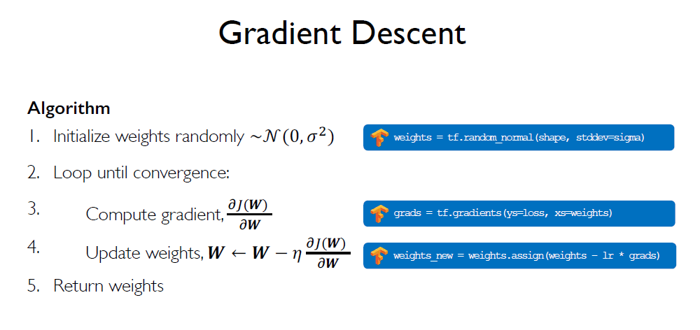gradient_descent fig: Gradient Descent

Since W is a matrix of the weights if inputs and weights of hidden layers, the update travels back through for every weight in the matrix. The following equations gives us the idea.

\[\begin{align*} & \frac{\partial J(W)}{\partial w_2} = \frac{\partial J(W)}{\partial \hat{y}} \frac{\partial \hat{y}}{\partial w_2} \\ & \frac{\partial J(W)}{\partial w_1} = \frac{\partial J(W)}{\partial \hat{y}} \frac{\partial \hat{y}}{\partial z_1} \frac{\partial z_1}{\partial w_1} \\ \end{align*}\]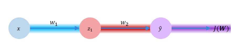

backpropagation

Training in Practice

Training Neural Networks are hard, usually because of the landscape of the cost function. Also there are several other hyper parameters that come into play like Learning rate, Overfitting and Underfitting, etc.

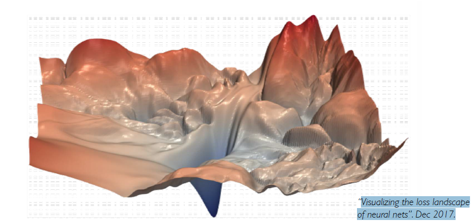landscape_of_loss fig: Complex topology of the loss landscape

Adaptive learning

The learning rate \(\eta\) can be tricky to set. A large learning rate results in cost function diverging from the minima, where as the small learning rate results in too many iterations for the cost function to converge. Many a time the usual approach adopted in practice is to try different learning rate and use one that best fits the problem. But this is computationally intensive and takes a lot of time.

Instead what we could have is a learning rate that adopts the landscape of the problem. Thus we need not have a learning rate that is not fixed. We could have the learning rate that could change depending on the how large the gradient is, how fast the learning is happening, size of the particular weights, etc. The figure below are some of the Adaptive Learning rates that are commonly used in TensorFlow.

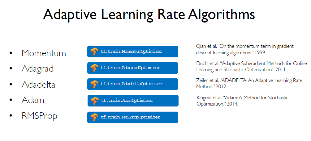adaptive_learning_rates fig: Some Adaptive Learning Rate Algorithms

Batching

Computing the cost function for every input of a training data can be computationally intensive task for very large data set. To address this problem Stochastic Gradient Descent was introduced, where a random training example is taken and the respective cost in computed and the weights are updated respectively. This is easy to compute but this also picks up a lot of noise in the data.

So instead of choosing a single training data point, we can choose a mini-batch of data point at random. Compute the cost of the mini-batch as the equation below and update the weights for the mini-batch. This is faster to compute and a much better estimate of the true gradient. This also gives us a smother convergence and allows for a larger learning rate. The mini-batches leads to faster training as they are parallelizable and using GPU’s leads to much faster training.

\[\begin{align*} \frac{\partial J(W)}{\partial W} = \frac{1}{B} \sum_{k=1}^B \frac{\partial J_k(W)}{\partial W} \end{align*}\]

where B is the size of the randomly chosen mini-batch.

Regularization

If a neural network is allowed to train on training data for a very long time it starts to learn very complex models which does not generalize well and gives a lot of errors on unseen data. To address this we employ Regularization. Regularization is a technique that constrains our optimization problem to discourage complex models. It improves generalization of our model on unseen data. There are two ways we can enforce regularization to our model.

Dropout

Here we randomly choose some percentage of nodes in the network and set them to 0(Typically 50% of the activation nodes in the network). This forces the network to not rely on any particular node in the network.

tf.keras.layers.Dropout(p=0.5)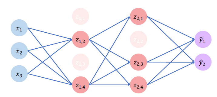

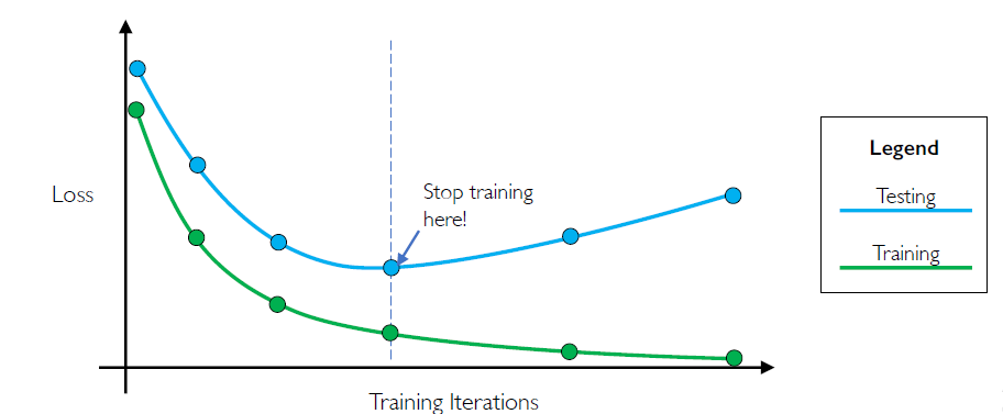
dropout

Early Stopping of training

We can stop training before the model has a chance to overfit the training data.

stop_training

This concludes this post on the Introduction to Deep Learning. In the Next post on deep learning we will look into Recurrent Neural Networks(RNN).

Nikhil